SheeplzSubscribe
Options pricing, made visible: The Price of a Shape
By Dylan Siegel
This is my understanding, for education. Not personal financial advice.
An option turns a future outcome into a contract you can buy today. Its price connects the shape of the payoff, the uncertainty before expiration, and what people will pay to transfer that risk.
That is the subject of The Price of a Shape. The film makes the mechanisms visible. This companion works through the economics and the arithmetic: where time value comes from, how implied volatility packages a price, why a correct directional call can still lose money, and what separates a useful forecast from a convincing backtest.
New to this? Read first: what a share represents and how market drawdowns work. The examples below are constructed teaching examples, not current quotes or recommendations. Prices are per share unless a contract amount is specified.
Watch the film
Open the full 19-minute film on YouTube. Select 2160p for 4K.
1. Start with the contract’s payoff
A call gives its owner the right to buy the underlying at a specified strike price. A put gives the right to sell. The expiration date fixes the contract’s horizon. Exercise and settlement rules determine how the right is used and what changes hands. These are part of the product, not fine print to add after pricing it. OIC: options basics.
Write the strike as K and the underlying price at expiration as ST. A call’s expiration value is the amount by which the underlying finishes above the strike. A put’s is the amount by which it finishes below.
Call payoff = max(ST − K, 0)
Put payoff = max(K − ST, 0)
Those are payoffs. Profit also accounts for what you paid. Buy a $100-strike call for $4 and the expiration profit is max(ST − 100, 0) − 4, before financing and trading costs.
| Final stock price | Call payoff | Buyer’s profit |
|---|---|---|
| $90 | $0 | −$4 |
| $100 | $0 | −$4 |
| $102 | $2 | −$2 |
| $104 | $4 | $0 |
| $110 | $10 | +$6 |
A standard, unadjusted U.S. equity option generally covers 100 shares. In that case, $4 quoted means $400 for one contract, and the $6 profit in the last row means $600. Adjusted contracts and other products can have different deliverables or multipliers. Always read the contract specification.
A straddle combines a call and a put at the same strike and expiration. Its payoff is |ST − K|. If the two options cost $8 together, a $100 straddle breaks even at $92 and $108 at expiration, before costs. A move in either direction helps, but a move smaller than the premium still leaves a loss. The size of the move and the price paid belong in the same sentence.
2. Time value is the value of unresolved possibilities
At a particular moment, a call’s intrinsic value is max(S − K, 0). Its quoted premium minus that intrinsic value is commonly called time value or extrinsic value. If a $100-strike call trades for $7 while the stock is $105, $5 is intrinsic and $2 is extrinsic. OIC: the components of option prices.
The name can be misleading. Time does not produce value by itself. It allows an uncertain future to unfold before the payoff becomes fixed. In the film, grains settle into the gap between today’s option value and its immediate-exercise value. That gap prices the possibilities still open.
Consider a deliberately simple, zero-interest example. The stock is $100 and the strike is $100. If the terminal price is certainly $100, the call pays nothing. If instead the terminal price is $90 or $110 with equal pricing weights, the average stock price is still $100, but the average call payoff is $5. The downside stops at zero; the upside keeps growing.
This is convexity. The average payoff of a curved function can exceed the payoff at the average input. More precisely, a mean-preserving spread of outcomes cannot reduce the expected payoff of a convex claim, and can raise it. A larger variance by itself does not completely order arbitrary distributions; their other features matter too.
Under a constant-volatility, zero-rate, zero-dividend Black–Scholes example, a $100 at-the-money call at 20% annualized volatility is worth about $2.287 with 30 calendar days left and $1.105 with seven days left. These are calculated model values, with the underlying held fixed. The call has zero intrinsic value in both cases.
Time value is not a separate payment the buyer receives back. It is embedded in the contract price. And the simple “premium is always above spot intrinsic value” intuition needs care for European contracts, which cannot be exercised early: rates, dividends and the restriction on exercise affect the comparison.
3. A probability forecast and a pricing distribution do different jobs
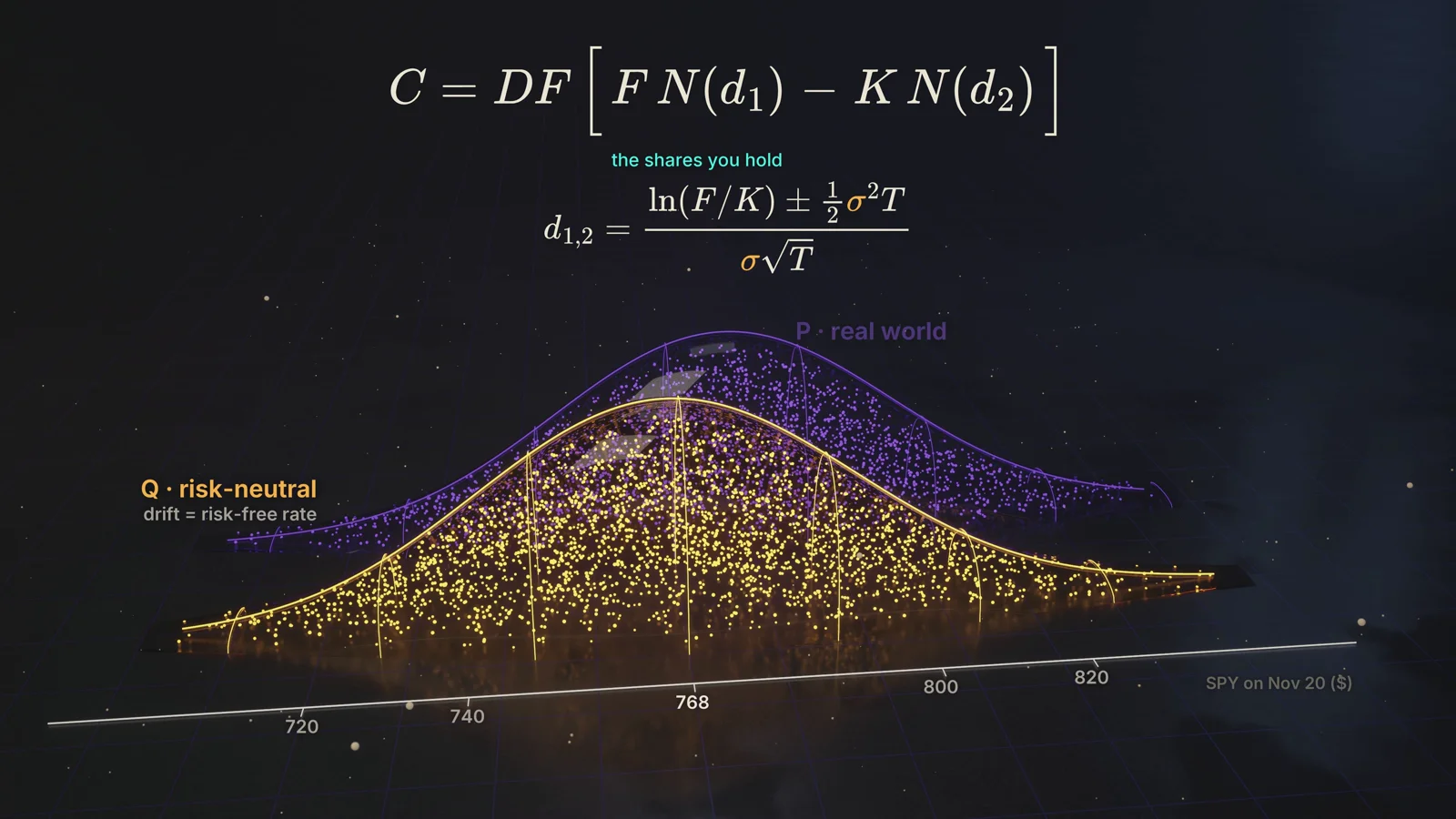
A physical probability, usually labelled P, describes how often you expect an outcome to occur. A risk-neutral probability, labelled Q, is a weight used to price a payoff consistently with traded assets. Q includes the market’s valuation of resources across future states. It is not a claim that investors are indifferent to risk. The Minneapolis Fed explains this distinction.
For a European payoff with a deterministic interest rate, the pricing relationship is:
Value today = e−rT × EQ[payoff at T]
Here r is the continuously compounded annual interest rate, T is years remaining, and E means a weighted average. The discount factor translates a future payment into today’s money. The superscript Q specifies which weights belong in the average.
A two-state example you can replicate
Suppose the stock costs $100 today and can finish at either $90 or $110. Assume no interest, no dividend, no costs, and the ability to trade fractional shares, sell short and borrow. A $100-strike call pays $0 or $10.
Buy half a share for $50 and borrow $45. Your net cost is $5. At expiration, the half-share is worth either $45 or $55. Repaying $45 leaves exactly $0 or $10: the call’s payoff in both states.
| At expiration | Stock at $90 | Stock at $110 |
|---|---|---|
| Half a share | $45 | $55 |
| Repay borrowing | −$45 | −$45 |
| Net payoff | $0 | $10 |
| Call payoff | $0 | $10 |
In this model, the call must cost $5. Otherwise, trading the cheaper version against the more expensive identical payoff would create an arbitrage. The pricing weight on the up state is 50% because 0.5 × $90 + 0.5 × $110 = $100.
You might personally forecast a 60% chance of the up state. Your expected call payoff would then be $6. That can inform whether you want the exposure. It does not change the cost of replicating the contract in this two-state market.
Real markets have jumps, trading constraints and risks that cannot all be replicated. The clean example explains why option prices cannot simply be built from someone’s unadjusted frequency forecast. Insurance paying during a market crash can command a high price because it pays precisely when money is particularly valuable.
4. Black–Scholes is a pricing model; implied volatility runs it backward
The Black–Scholes model connects a European option’s price to the underlying, strike, time, interest rate and volatility. A common extension includes a continuous dividend yield. Its idealized setup assumes continuous price paths, constant volatility and rates, and frictionless dynamic hedging. Replication is the central idea. The stock’s expected excess return disappears from the pricing equation because the model hedges the stock exposure. MIT: risk-neutral valuation and Black–Scholes.
The formula, with the symbols defined
C = S e−qTN(d1) − K e−rTN(d2)
d1 = [ln(S/K) + (r − q + σ²/2)T] / (σ√T)
d2 = d1 − σ√T
C is the call price; S is the underlying price; K is the strike; r is the interest rate; q is the continuous dividend yield; σ is annualized volatility; T is years to expiry; N is the standard normal cumulative distribution function. Enter 20% volatility as 0.20. The examples here use T = calendar days / 365 and r = q = 0 unless stated otherwise.
The European put follows from put–call parity: P = C − S e−qT + K e−rT. At zero rates and dividends, a call minus a put has the same expiration payoff as stock minus the strike amount in cash. This is a consistency relationship between prices, not a prediction of direction. OIC: put–call parity.
Given a volatility assumption, the model produces a theoretical price. Given a market price, you can solve for the volatility that reproduces it. That second operation gives implied volatility, or IV.
Suppose the $100, 30-day call trades at the model’s $2.287. With zero rates and dividends, its IV is 20%. If the quote rises while the other inputs are unchanged, the IV rises too. Saying “the option rose because IV rose” can therefore be an accounting description of the same price change, not an independent explanation of what caused it.
IV is useful because it lets people compare differently priced contracts in a common language. But it is conditional on a model and its inputs. Different strikes and expirations can imply different volatilities. A single number cannot describe every tail, event or path the market is pricing.
The exercise style matters. American options can be exercised before expiration and usually need an early-exercise-capable model, such as a suitable binomial tree. Discrete dividends, borrow costs and settlement mechanics also matter. A precise formula with the wrong contract assumptions can give a precise wrong answer. OIC: pricing models and their limits.
5. The Greeks explain how the price can change
The Greeks are local sensitivities of a model price. Each asks what happens when one input changes while the others are held fixed. They are estimates around the current state, not guarantees about the next market quote. OIC: understanding the Greeks.
| Greek | Question | A quoted example |
|---|---|---|
| Delta, Δ | How much does the option change for a small change in the underlying? | 0.50 suggests about +$0.50 for a $1 rise. |
| Gamma, Γ | How quickly does delta change? | 0.04 suggests delta rises about 0.04 after a $1 rise. |
| Theta, Θ | What is the effect of time passing? | −0.03 per day suggests about $0.03 of daily decay. |
| Vega | How does the price respond to a change in IV? | 0.12 per volatility point suggests +$0.12 when IV moves from 20% to 21%. |
| Rho | How does the price respond to a change in rates? | Check whether the quote is per percentage point or per unit rate. |
For a small move, a useful approximation is:
Change in option value ≈ Δ × ΔS + ½Γ × (ΔS)² + Θ × Δt + Vega × ΔIV
The capital Δ before S or IV means “change in”; the standalone Δ is the delta sensitivity. Match the units: daily theta needs days, and vega quoted per percentage point needs the change in volatility points. Rate changes, cross-effects and higher-order terms are omitted here. For a large move, reprice the whole option.
The stock rises, but the call loses value
Return to the $100-strike call. Start with the stock at $100, 30 days left and 20% IV. One day later, the stock rises to $101, but IV falls to 12%. Using the same zero-rate, zero-dividend model:
| Scenario | Inputs | Call value |
|---|---|---|
| Purchase | S = $100; 30 days; IV = 20% | $2.287 |
| Next day, IV unchanged | S = $101; 29 days; IV = 20% | $2.795 |
| Next day, IV falls | S = $101; 29 days; IV = 12% | $1.914 |
The directional forecast was right. The option still lost about $0.373 per share, or $37.30 for a 100-share contract before costs. A change in the price of uncertainty outweighed the benefit from the stock move.
Delta is also not a universal probability of profit. In the no-dividend Black–Scholes model, call delta is N(d1), while the risk-neutral probability of expiring in the money is N(d2). Neither includes your premium in a break-even test, and neither is automatically your physical probability forecast.
6. Gamma and theta are two sides of a pricing balance
A plain long call or put is convex: its delta adjusts favorably as the underlying moves. That is positive gamma. Short-dated options near the strike can have particularly high gamma because small underlying moves can rapidly change whether the contract is likely to finish in the money. OIC: gamma and expiration.
In the constant-volatility Black–Scholes model, with elapsed-time theta expressed per year and a continuous dividend yield q, the pricing equation can be written as follows. V is the option’s value.
Θ + ½σ²S²Γ + (r − q)SΔ − rV = 0
Set rates and dividends to zero and it reduces to Θ = −½ΓS²σ². The model’s cost of waiting balances the value of curvature under its assumed variance. This is the identity shown in the film. It is not a universal statement that every option’s quoted theta equals that simplified expression in every market. MIT: the Black–Scholes pricing equation.
Reproducing the film’s arithmetic
The on-screen example uses gamma 0.0156, underlying price $765.90 and annualized volatility 13.58%. Under the zero-carry simplification:
Daily theta ≈ −½ × 0.0156 × 765.90² × 0.1358² ÷ 365
≈ −$0.2312 per share per calendar day
For a 100-share contract that is about −$23.12 per day at that instant, holding the inputs fixed. It is not a promise that tomorrow’s market price will fall by $23.12. Spot, IV and gamma can all change; the rate of decay changes with them.
Why movement can pay for decay
Imagine holding a long option and offsetting its current delta with stock. Over a small step, at zero rates and dividends and ignoring costs and IV changes, the position’s approximate gain is:
Hedged gain ≈ ½Γ[(ΔS)² − S²σimplied²Δt]
Here Δt is a fraction of a year and σ is decimal annualized volatility.
This follows by subtracting the delta term and inserting the simplified theta identity. It compares the movement actually delivered with the movement priced into the option. The gamma changes along the path, so an option trade effectively weights realized movement differently at different times. Simply comparing two headline annualized volatilities is not a complete profit calculation.
Continuous, costless hedging is an assumption. Real hedges happen at discrete times, pay spreads and can miss jumps. The formula explains the exposure; it does not remove execution risk.
7. Measure movement on the same clock
Volatility is the square root of variance. For short return intervals, a common realized-variance measure adds squared log returns:
ri = ln(Si / Si−1)
Realized variance over the window = Σ ri²
Taking the square root gives a realized-volatility measure for that window. Annualization then depends on its length and convention. Overnight returns, jumps, sampling frequency and noisy quotes change what you are measuring. More frequent observations do not automatically produce a better estimate: bid–ask bounce and other microstructure effects can contaminate the sum. Federal Reserve research: measuring realized variance.
The path matters for this measurement. A stock that goes from $100 to $105 and back to $100 has approximately zero net return, but its two nonzero returns contribute positive realized variance. An unhedged call held to expiration can nevertheless finish worthless. A delta-hedged option follows a different cash-flow path. “The market moved a lot” needs a definition and a trading rule.
Under a simple constant-variance diffusion, a rough one-standard-deviation dollar scale is S × σ × √T. For S = $100, σ = 20% and T = 30/365, it is about $5.73. This is a model scale, not a guaranteed trading range or a promised 68% coverage rate in real markets.
Twenty percent annualized on a 252-trading-day convention implies about 1.26% for one trading day. Dividing the same quoted number by √365 gives about 1.05% for a calendar day. These are different time conventions. Do not compare an intraday estimate with a calendar-time option quote until the horizon, overnight treatment and units agree.
The deeper idea behind a variance clock is to track how much squared movement has accumulated rather than counting equal minutes. An opening auction, a quiet lunch hour and a data release need not spend the same amount of variance. A normalized clock might divide variance delivered so far by the variance budget expected for the full window. That can describe a market state; it becomes a trading signal only after testing whether it predicts something useful.
One more horizon trap: VIX represents a constant 30-day option-implied measure derived from SPX options. It is not the IV of every option and is not interchangeable with a forecast for the next 15 minutes. Cboe: why the volatility horizon matters.
8. The smile contains information a single volatility cannot
Take options on the same underlying with the same expiry and calculate IV at each strike. A flat line would be consistent with the simplest constant-volatility model. Actual quotes often form a smile or a skew. In equity indexes, out-of-the-money puts commonly trade at higher IV than comparably distant out-of-the-money calls. Cboe: equity-index skew.
That pattern describes relative prices across outcomes. It is influenced by the distribution being priced, demand for downside protection and the cost of supplying it. It does not let you uniquely separate “fear,” expected crashes and dealer constraints from one snapshot.
A 25-delta put and a 25-delta call are points on a surface, not permanent fixed contracts. If spot or volatility moves, the strikes corresponding to those deltas can move too. A change in a delta-based skew measure and a change in the IV of a fixed-strike option answer related but different questions.
How prices reveal a distribution
For smooth European call prices C(K,T), deterministic rates and suitable no-arbitrage conditions, the Breeden–Litzenberger relationship is:
Risk-neutral density at K = erT × ∂²C(K,T) / ∂K²
This is curvature across strike, holding today’s underlying price fixed. Gamma is curvature across the underlying price, holding the contract fixed. Confusing the two loses the meaning of the formula.
A narrow butterfly makes the relationship tangible. Buy calls at K − h and K + h, and sell two calls at K. The resulting expiration payoff is a small tent centered on K. Its price samples how much the market charges for outcomes near that strike. As the tent narrows, properly scaled prices reveal the density.
The film’s sand pile is a way to visualize those pricing weights. Estimating the pile from real quotes requires smoothing, synchronized prices, suitable exercise adjustments and no-arbitrage checks. Differentiating noisy quotes twice can create negative “probabilities.” The far tails also require assumptions where strikes are scarce. Allan Malz’s New York Fed paper explains the estimation problem.
9. Calendar time and event risk are not interchangeable
An expiration before a scheduled announcement and one after it contain different uncertainty. An earnings release or election can concentrate a large amount of potential movement into a short interval. Spreading that uncertainty evenly across every remaining day hides the mechanism.
For a simple illustration, let background annual volatility be 20%, and add one independent, zero-mean event return with a 3% standard deviation. The event contributes 0.03² to total return variance. If the expiry includes that event, the variance budget is:
Total variance = 0.20² × T + 0.03²
Equivalent annualized volatility = √(total variance / T)
| Time left | Background volatility | Equivalent volatility with event |
|---|---|---|
| 7 calendar days | 20% | 29.48% |
| 30 calendar days | 20% | 22.57% |
The event has not become more violent in the seven-day example. Its fixed variance is being annualized over less time. This is variance bookkeeping, not an exact calibration of every option’s IV: a discrete jump distribution can affect strikes differently.
After the event, that unresolved-event component disappears. IV can fall even if the price makes the move you expected. It can also remain elevated if the event creates new uncertainty. The outcome and the repricing of what remains uncertain are separate inputs to your option’s value.
Subtract total variance, not volatility percentages
For compatible variance quotes, write W(T) = σ(T)²T. The implied average variance between two maturities is [W(T2) − W(T1)] / (T2 − T1). With 30-day volatility of 20% and 60-day volatility of 22%, the forward volatility for days 30–60 is:
√[(0.22² × 60 − 0.20² × 30) / 30] ≈ 23.83%
The answer is neither 2% nor 22%. This calculation is cleanest for consistently defined variance measures. Applying it to at-the-money Black–Scholes IVs is an approximation; changing forwards, skew and event distributions can matter. CME’s event-volatility tools use term and forward volatility to examine the uncertainty around scheduled events. CME: event volatility.
Weekends are another clock problem. Markets can account for expected non-trading time in the prices quoted before the closure, and different models allocate that time differently. Three calendar days do not create three days of guaranteed seller profit. News can arrive while the hedge market is closed. OIC: theta and weekend conventions.
10. The option seller earns a premium by taking an obligation
The buyer’s premium becomes the seller’s cash receipt, but the seller also assumes a liability. Receiving cash is not the same as realizing a profit. The position must be bought back, expire or settle, and its risk may require capital or collateral in the meantime.
At matched horizons, one common definition of the variance risk premium is the risk-neutral expected variance minus the physical expected variance. A positive gap means variance exposure is priced above its expected realized amount under the physical forecast. Researchers use this distinction to separate priced uncertainty from statistical expectations. Sign conventions differ across papers, so read the definition. Bali and Zhou: definition and measurement of the variance risk premium.
Suppose a consistently defined implied variance measure corresponds to 24% annualized volatility and your same-horizon physical forecast corresponds to 18%. The variance gap is 0.24² − 0.18² = 0.0252 per year. It is not the six-point volatility difference, and it is not a 2.52% guaranteed return on capital. A trade’s dollars depend on its exposure, horizon, hedge, costs and payoff.
A single option’s Black–Scholes IV is not the same object as a model-free variance-swap measure. Nor is yesterday’s realized volatility automatically the correct forecast for tomorrow. Comparing the wrong objects can manufacture an apparent premium.
A high win rate can conceal a losing payoff
Consider 100 hypothetical trades: 95 earn $1 each and five lose $25 each. The win rate is 95%, but the total is $95 − $125 = −$30 before costs. Frequent small receipts say little about the price of the rare obligation.
Protection can be worth buying even when its standalone average return is negative. A put that pays during a damaging portfolio drawdown can provide insurance, liquidity or the ability to avoid a forced sale. The buyer and seller may value that same exposure differently because their other assets and constraints differ.
For the seller, the relevant questions include the size of a bad loss, the ability to finance it, the cost of closing when spreads widen and whether a hedge survives a gap. Covered calls, cash-secured puts and uncovered options create different portfolios. The premium alone does not describe any of them.
11. A useful forecast must improve an actual decision
A forecast can predict direction, a variance rate, a terminal distribution, a jump probability or a future volatility surface. These are different targets. A strong forecast for the next 15 minutes can still be poorly matched to an option held until a later expiration.
For a trade exited before expiry, you must value the contract at the exit state. Its remaining time value has not vanished. A scenario engine therefore needs more than a terminal stock price: it needs assumptions about remaining IV, skew, time, rates and exercise where relevant. The film’s flowing forecast paths are a useful picture of possibilities, but the pricing rule applied at each path’s exit determines the resulting profit distribution.
Correlation is only one diagnostic. If a forecast is exactly twice the realized quantity in every observation, it can have perfect correlation and still be badly miscalibrated. Directional accuracy can also be high while the largest misses dominate the money lost.
| Test | What it reveals |
|---|---|
| Same horizon and units | Whether the forecast and target measure the same thing. |
| Calibration | Whether predicted levels and probability ranges agree with outcomes. |
| Simple benchmarks | Whether complexity improves on recent volatility, time of day or market prices. |
| Tail behavior | What happens during jumps, large losses and unusual sessions. |
| Executable trading simulation | Whether an advantage survives spreads, fees, delay and the exit rule. |
A small valuation advantage can disappear in the spread
Suppose an option is quoted $2.00 bid and $2.10 ask. Your model says $2.12. The midpoint is $2.05, so a midpoint comparison advertises a seven-cent advantage. An immediate buyer pays $2.10, leaving only two cents before commissions, adverse movement and exit costs. On a 100-share contract that is $2, not $7.
If your plan requires buying at the midpoint, the simulation must explain when that order fills and what happens when it does not. A favorable theoretical mark is not an executed trade. The same discipline applies to a multi-leg spread: synchronized quotes, leg execution and liquidity all belong in the calculation.
A forecast’s value is the improvement it makes to a defined decision after these constraints. It might improve hedging or position selection without being strong enough to support a standalone trade. That is still useful information.
12. Read the evidence grade as carefully as the result
The film labels illustrative scenes and grades research claims. The spot-volatility scatter, hourly realized-volatility series and buyer/seller distributions described as illustrative explain mechanisms. Their shapes are not substitutes for a measured dataset.
A selected historical week is a vignette: it can show what a mechanism looked like. An in-sample relationship describes data already used during development. A test on genuinely untouched future data asks a harder question. These categories should not be blended into one claim of proof.
Trying many settings creates a selection problem. The best-looking backtest can be the one most fitted to the noise. Reusing the same “test” period after every adjustment gradually turns it into development data. Bailey and co-authors study this problem directly in The Probability of Backtest Overfitting.
For a short-window options study, I want to see the split dates, when each feature was available, how many variants were tried, and how fills were simulated. Overlapping forecast windows also share outcomes: thousands of rolling observations do not automatically provide thousands of independent pieces of evidence.
Results should show their concentration. Report performance by day and underlying, the contribution of the largest gains and losses, drawdowns, and sensitivity to realistic costs. Removing the best day is a stress test of dependence, not a proof that the remaining strategy is valid. A market shock can be both a legitimate source of payoff and the reason the sample is too narrow to support a broad claim.
The next useful test freezes the rules before new observations arrive. A failing result should change the conclusion, not merely trigger another search on the same period. The educational sources in this article support the pricing concepts; they do not independently validate the film’s empirical research.
Put the pieces together before judging a trade
A complete option thesis has to connect the contract, the forecast and the price. Start with the payoff and expiration. Identify the event window. Read the relevant strike and expiry on the surface. Then specify what you expect to change, when you will exit, and how that exit value will be calculated.
For a long call, “the stock will rise” leaves several questions unanswered. How far and how soon? What premium is already being paid for that possibility? Will IV fall after an event? What happens if the rise arrives after expiry? Does a modest favorable outcome cover the spread? A short option requires the corresponding questions about losses, hedging, assignment and capital.
The film’s central shape is therefore more than an expiration diagram. It is a payoff evaluated across possible futures, priced with market weights, and carried through time under changing conditions. Understanding that connection makes an option quote easier to interpret—and makes it harder to mistake a persuasive story for a favorable trade.
Questions worth settling
Does high IV mean an option is expensive?
It means the quoted price maps to a high volatility input under the chosen model. “Expensive” needs a comparison: the same horizon’s plausible future movement, tail and event risks, other strikes or maturities, and the cost of taking the position. A low dollar premium can still be expensive relative to what the contract is likely to pay.
Does an option need to cross its expiration break-even before I can sell it for a profit?
No. Before expiration, its resale value still includes remaining time and uncertainty. A call can increase in price while the underlying remains below K plus the original premium. The expiration break-even describes holding to expiry, not every earlier exit.
Does delta neutrality eliminate risk?
No. It offsets the first-order response to a small underlying move at the current state. Gamma changes that exposure; IV and time can move the value; a jump can cross a large price interval before you rebalance. The hedge itself has execution and financing costs.
What changes for same-day expiration?
The remaining time is short, so gamma and theta can be concentrated around the strike. A small timing error or a missed hedge can have a large effect relative to the premium. A model using calendar days should represent the fraction of a day remaining; rounding the entire session to zero destroys the time input.
Are stock, ETF and index options interchangeable?
No. Exercise style, physical versus cash settlement, the settlement calculation and the multiplier can differ. Many U.S. stock and ETF options are American-style with share delivery; many index options are European-style and cash-settled. Verify the particular product, including its settlement time. OIC: equity and index contract differences.
Return to the film with the pricing mechanics in mind ↑
Sources, assumptions and further reading
Worked dollar examples are original calculations for this article, except the explicitly identified gamma–theta inputs shown in the film. The model examples use European exercise, zero interest and dividends, and actual calendar days divided by 365. They exclude trading costs unless a cost is the subject of the example.
- Options Industry Council: Options Basics and Options Pricing — contracts, premiums and intrinsic value.
- Federal Reserve Bank of Minneapolis: Market-Based Probabilities — what pricing probabilities mean.
- MIT OpenCourseWare, Lecture 21: Black–Scholes and Risk-Neutral Valuation — replication and valuation.
- OIC: Black–Scholes Formula and Put/Call Parity — model inputs and consistency between payoffs.
- OIC: Understanding Options Greeks, with its linked Delta, Gamma, Theta and Vega explanations — local sensitivities and conventions.
- MIT OpenCourseWare, Lecture 24, slides 4–8 — dynamic hedging and the Black–Scholes equation.
- Hao Zhou: Variance Risk Premia, Asset Predictability Puzzles, and Macroeconomic Uncertainty, 2010, section 2 — implied and realized variance measurement.
- Cboe: VIX and VIX1D — volatility horizons.
- Cboe: The Adventures of Volatility Markets — equity-index skew.
- Allan M. Malz: A Simple and Reliable Way to Compute Option-Based Risk-Neutral Distributions, Staff Report 677, 2014 — density extraction and no-arbitrage restrictions.
- CME Group: Event Volatility Calculator — term structure and event analysis.
- Turan G. Bali and Hao Zhou: Risk, Uncertainty, and Expected Returns, 2011, section 2.1 — the variance risk premium.
- Bailey, Borwein, López de Prado and Zhu: The Probability of Backtest Overfitting, 2015 — selection and repeated testing.
- OIC: Equity vs. Index Options — exercise and settlement.
The film’s illustrations and short research samples should be interpreted with their on-screen evidence labels. This article explains the mechanisms and adds examples; it does not claim a newly validated trading strategy.